R Transformation
R transformations are for advanced statistical computations. Apart from ready-to-use implementations of state-of-the-art algorithms, R’s other great assets are vector and matrix computations. R transformations complement Python and SQL transformations where computations or other operations are too difficult. Common data operations like joining, sorting, or grouping are still easier and faster to do in SQL Transformations.
Environment
Section titled “Environment”The R script is executed in an isolated environment. The current R version is 4.0.5, however it is possible to switch your configuration to run on other versions if available.
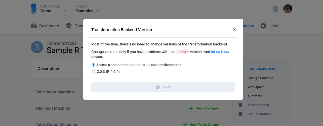
Any updates to the R version is always announced in the Keboola changelog.
Memory and Processing Constraints
Section titled “Memory and Processing Constraints”An R transformation has a limit of 16GB of allocated memory and the maximum running time is 6 hours. The CPU is limited to the equivalent of two 2.3 GHz processors.
File Locations
Section titled “File Locations”The R script itself will be compiled to /data/script.R. To access your
mapped input and output tables, use
relative (in/tables/file.csv, out/tables/file.csv) or absolute (/data/in/tables/file.csv, /data/out/tables/file.csv) paths.
To access downloaded files, use the in/files/ or /data/in/files/ path. If you want to dig really deep,
have a look at the full Common Interface specification.
Temporary files can be written to a /tmp/ folder. Do not use the /data/ folder for those files you do not wish to exchange with Keboola.
R Script Requirements
Section titled “R Script Requirements”You can organize your script into blocks, but the resulting R script to be run within our environment must meet the following requirements:
Packages
Section titled “Packages”The R transformation can use any package available on
CRAN. In order for a package and
its dependencies to be automatically loaded and installed, list its name in the package section. Using library()
for loading is not necessary then.
The latest versions of packages are always installed. Some packages are pre-installed in the environment
(see list). These pre-installed packages are
installed with their dependencies, therefore to get an authoritative list of installed packages use the installed. packages() function. It does no harm if you add one of these packages to your transformation explicitly, but the transformation and
sandbox startup will be slowed by the forced re-installation.
CSV Format
Section titled “CSV Format”Tables from Storage are imported to the R script from CSV files. The CSV files can be read by standard R functions.
Generally, the table can be read with default R settings. In case R gets confused, use the exact format
specification sep=",", quote="\"". For example:
data <- read.csv("in/tables/in.csv", sep=",", quote="\"")Row Index in Output Tables
Section titled “Row Index in Output Tables”Do not include the row index in the output table (use row.names=FALSE). If you are using the
readr package, you can also use the write_csv function
which doesn’t write row names.
write.csv(data, file="out/tables/out.csv", row.names=FALSE)The row index produces a new unnamed column in the CSV file which cannot be imported to Storage. If the row names contain valuable data, and you want to keep them, you have to convert them to a separate column first.
df <- data.frame(first = c('a', 'b'), second = c('x', 'y'))data <- cbind(rownames(df), df)write.csv(data, file="/data/out/tables/out.csv", row.names=FALSE)Errors and Warnings
Section titled “Errors and Warnings”We have set up our environment to be a little zealous; all warnings are converted to errors and they cause the
transformation to be unsuccessful. If you have a piece of code in your transformation which may emit warnings,
and you really want to ignore them, wrap the code in a tryCatch call:
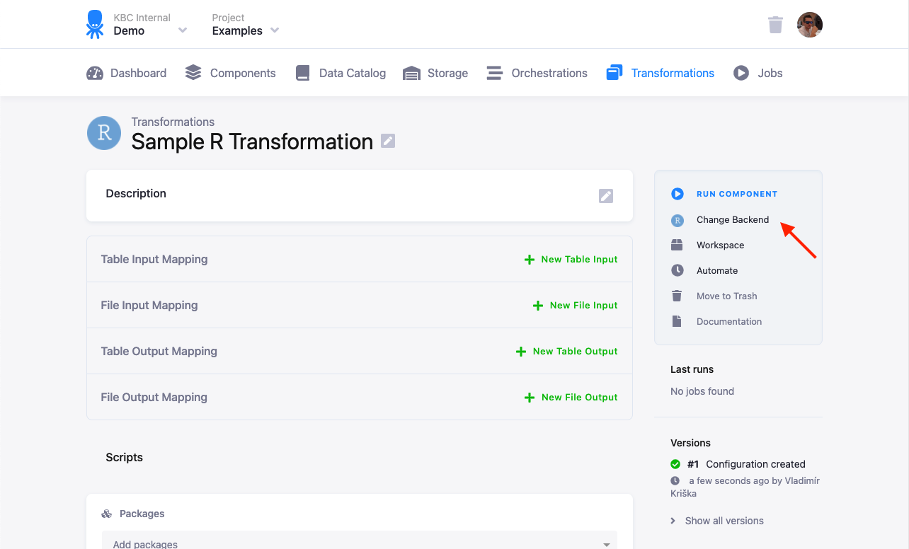
tryCatch({ ... some code ... },warning = function(w) {})Dynamic Backends
Section titled “Dynamic Backends”If you have a large amount of data in databases and complex queries, your transformation might run for a couple of hours. To speed it up, you can change the backend size in the configuration. R transformations support the following sizes:
- XSmall
- Small (default)
- Medium
- Large
Scaling up the backend size allocates more resources to speed up your transformation, which impacts time credits consumption.
Development Tutorial
Section titled “Development Tutorial”We recommend that you create an R Workspace with the same input mapping your transformation will use. This is the fastest way to develop your transformation code.
mydata <- read.csv("in/tables/mydata", nrows=500)This will help you catch annoying issues without having to process all data.
You can also develop and debug R transformations on your local machine. To do so, install R, preferably the same version as us. It is also helpful to use an IDE, such as the Jupyter Notebook.
To simulate the input and output mapping, all you need to do is create the right directories with the right files. The following image shows the directory structure:
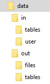
The script itself is expected to be in the data directory; its name is arbitrary. It is possible to use relative directories,
so that you can move the script to a Keboola transformation with no changes. To develop an R transformation which takes
a sample CSV file locally, take the following steps:
- Put the R code into a file, for instance, script.R in the working directory.
- Put all tables from the input mapping inside the
in/tablessubdirectory of the working directory. - Place the binary files (if using any) inside the
in/usersubdirectory of the working directory, and make sure that their name has no extension. - Store the result CSV files inside the
out/tablessubdirectory.
Use this sample script:
data <- read.csv(file = "in/tables/source.csv");
df <- data.frame(col1 = paste0(data$first, 'ping'),col2 = data$second * 42)write.csv(df, file = "out/tables/result.csv", row.names = FALSE)
A complete example of the above is attached below in data.zip.
Download it and test the script in your local R installation. The result.csv output file will be created.
This script can be used in your transformations without any modifications.
All you need to do is
- create a table in Storage by uploading the sample CSV file,
- create an input mapping from that table, setting its destination to
source(as expected by the R script), - create an output mapping from
result.csv(produced by the R script) to a new table in your Storage, - copy & paste the above script into the transformation code, and finally,
- save and run the transformation.
Events and Output
Section titled “Events and Output”It is possible to output informational and debug messages from the R script simply by printing them out. The following R script:
print('doing something')Sys.sleep(3)print('doing something else')Sys.sleep(3)write('still doing something', stdout())Sys.sleep(3)write('error message', stderr())Sys.sleep(3)app$logInfo("information")Sys.sleep(3)app$logError("error")Sys.sleep(3)TRUEproduces the following events in the transformation job:
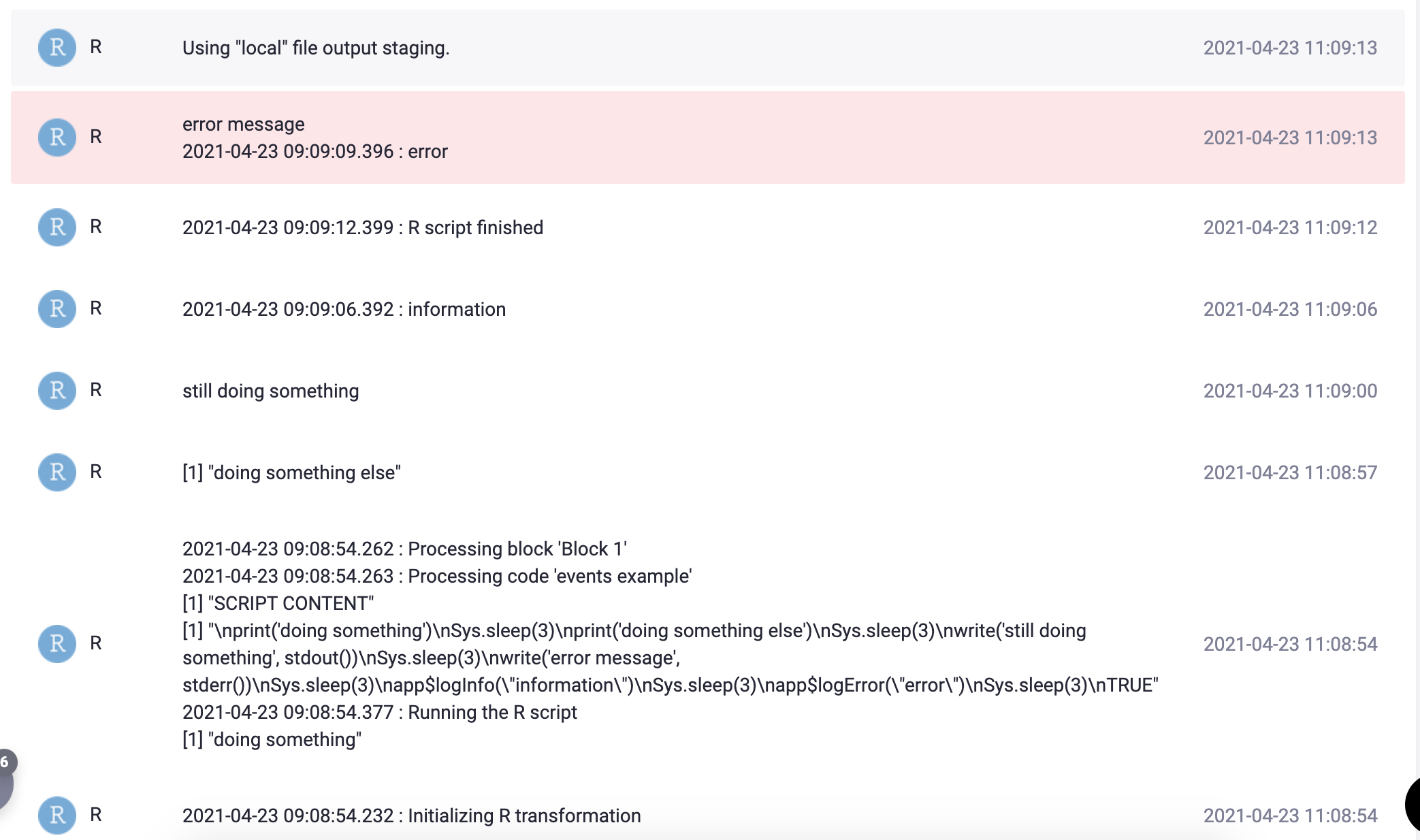
The app$logInfo and app$logError functions are also internally available; they can be useful if you need to know
the precise server time of when an event occurred. The standard event timestamp in job events is the time when the event was received
converted to the local time zone.
Going Further
Section titled “Going Further”The above steps are usually sufficient for daily development and debugging of moderately complex R transformations, although they do not reproduce the transformation execution environment exactly. To create a development environment with the exact same configuration as the transformation environment, use our Docker image.
Examples
Section titled “Examples”There are more in-depth examples dealing with