Input and Output Mapping
To configure input and output mappings in the process of creating a transformation, go to our Getting Started tutorial.
When manipulating your data, there is no need to worry about accidentally modifying the wrong tables. Mapping separates the source data from your transformation script. It creates a secure staging area with data copied from specified tables and brings only specified tables and files back to Storage. While the concept of mapping is most important for transformations, it actually applies to every single component.
Two mapping types must be set up before running a transformation:
- Input Mapping — This is a list of Storage tables used in your transformation.
If an input mapping does not fit well to your use case, then a read-only input mapping offers straightforward access to the data, and will drastically reduce the execution time.
This feature is useful in the following scenarios:
- Slow transformations where a clone is not used (input mapping)
- Complex orchestrations that move data from a data source to the workspace where they are accessed by other apps
- Cases where updating data in Storage via output mapping causes multiple data movement operations
- Output Mapping — This is a list of tables written into Storage after running the transformation. Tables not listed are neither modified nor permanently stored (i.e., they are temporary). They are deleted from the transformation staging area when the execution finishes.
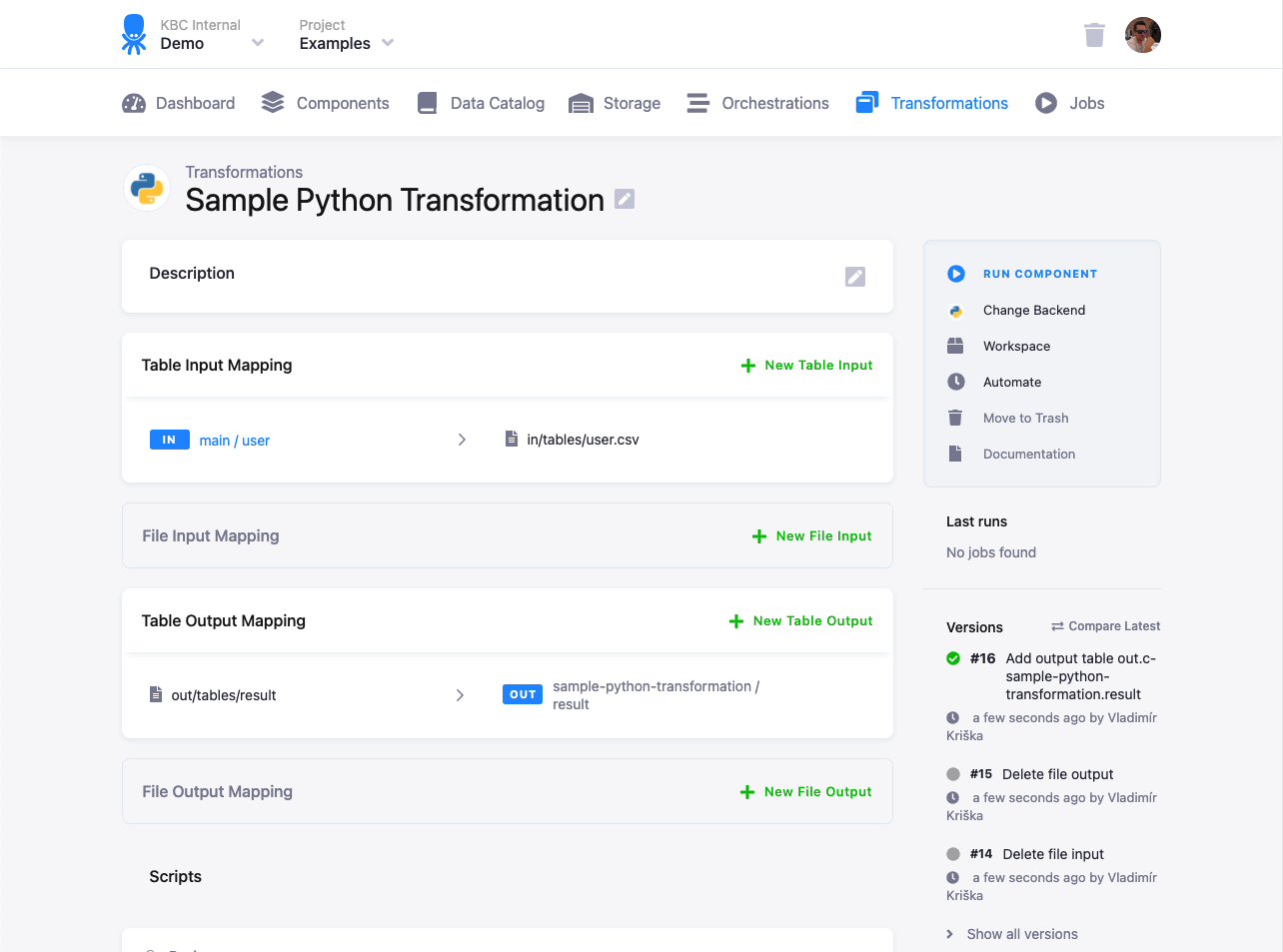
Table names referenced by mappings are automatically quoted by Keboola. This is especially important for Snowflake, which is case sensitive.
Overview
The concept of mapping helps to make the transformations repeatable and protect the project Storage. You can always rely on the following:
- Having an empty staging Storage (no need to clean up before transformations)
- Having an isolated staging Storage (no need to worry about interference with other transformations)
- Having a stateless transformation (no need to worry about having left-over variables and settings from something else)
- Resource cleanup (no need to worry about cleaning up temporary data after yourself)
- Resource conflict (no need to worry about naming data in the staging Storage)
While this makes some operations seemingly unnecessarily complicated, it ensures that transformations are repeatable and you can’t inadvertently overwrite data in the project Storage. For ad-hoc operations, we recommend you use workspaces. For bulk operations, consider taking advantage of variables and programmatic automation.
Input Mapping
Both Storage tables and Storage files can be used in the input mapping of a transformation. The common first choice is to use an input mapping with tables.
Table Input Mapping
Depending on the transformation backend, the table input mapping process can do the following:
- Database Staging: Copy the selected tables to tables in a newly created database schema. If you have not selected any tables and read-only input mappings are enabled, you can access them automatically in the workspace. In this case the tables are not copied.
- File Staging: Export the selected tables to CSV files and copy them to a designated staging Storage (not to be confused with a file mapping, as we’re still working with tables).
Depending on the transformation types, you can either build your transformations working with database tables or with CSV files. Furthermore, the CSV files can be placed locally with the transformation script or they can be placed on a remote storage such as Amazon S3 or Azure Blob Storage. The supported database type is Snowflake.
See an example of setting up an input mapping in our tutorial.
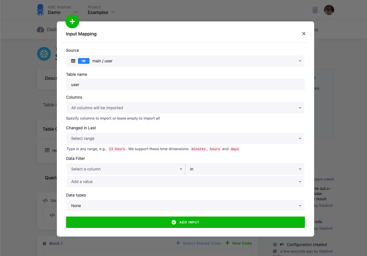
Options
When using table with native data types, following options will not be available.
- Source — Select a table or a bucket in Storage as the source table for your transformation. If you select a bucket, it is the equivalent of selecting all tables currently present in the bucket. It does not automatically add future tables to the selection.
- File name / Table Name — Enter the destination name of the mapping that is the Source table/file
name to be used inside the transformation. This is an arbitrary name you’d like to use as a reference for the table
inside the transformation script (it fills in automatically, but it can be changed). For File Staging, it is a good
idea to add the
.csvextension. For Database Staging, the table name is automatically quoted, which means you can use an arbitrary name. It also means that they may be case sensitive, for instance, if the destination is in Snowflake staging. - Columns — Select specific columns if you do not want to import them all; this saves processing time for larger tables.
- Changed in last — If you use incremental processing,
this comes in handy; import only rows changed or created within the selected time period.
The supported time dimensions are
minutes,hours, anddays. - Data filter — Filter source rows to the rows that match this single-column multiple-values filter. When used together with Changed in last, the returned rows must match both conditions.
- Data types — Configure data types.
If the terms source and destination look confusing, consult the image below. We always use them in a specific context. That means input mapping destination is the same file as the source for a transformation script.

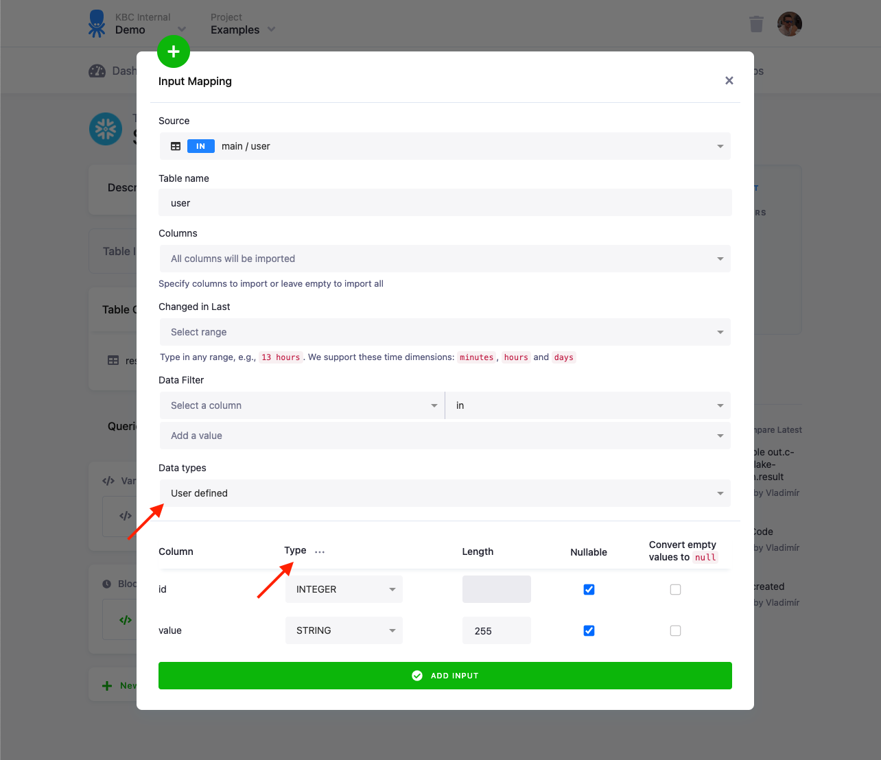
Data types
When selecting user defined data types the transformation jobs can take longer than usual because new typed table will be created in the background before materializing in output into final output table
The data types option allows you to configure settings of data types for the destination table. Data types are applicable only for destinations in database staging. Select User defined to configure data types for individual columns. The types are pre-configured with data types stored in the table metadata. The Type, Length, and Nullable options define the destination table structure in the staging database.
The option Convert empty values to null adds additional processing which is particularly important for non-string columns.
All data in Storage tables are stored in string columns, and empty values (be it true NULL values, or empty strings) are stored
as empty strings. When converting such values back to, for example, INTEGER or TIMESTAMP, they have to be converted to true
SQL NULL values to be successfully inserted.
The pre-set data types are only suggestions, you can change them to your liking. You can also use the three dots menu to bulk set
the types. Beware, however, that if a column contains values not matching the type, the entire load (and transformation) will
fail. In such a case, it’s reasonable to revert to VARCHAR types – for example, by setting Data types to None.
Snowflake loading type
When working with large tables, it may become important to understand how the tables are loaded into a Snowflake staging
database. We use two loading options: COPY and CLONE. The clone copy type is a highly optimized operation which
allows loading an arbitrary large table in near-constant time. There is a limitation, however, that the clone type can’t be used
together with any filters or data type configurations.
This might present a dilemma when loading huge tables. A logical approach when trying to speed up loading a large table would
be setting data types and adding filters to copy only the necessary ones. You might find out, however, that at some point, it’s
actually faster to remove the filters and data types, take advantage of the CLONE loading type, and apply the filters
inside the transformation. Also, when you need more complex filters (filtering by multiple columns or ranges), it’s best to
remove the filter completely from the input mapping, take advantage of the clone loading and do the filtering inside of the
transformation.
You can verify the table loading type in the events — copy table:
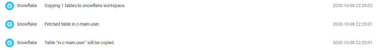
Clone table:
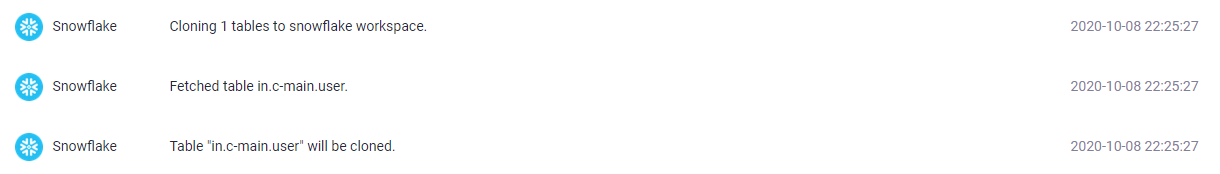
The CLONE mapping will execute almost instantly for a table of any size (typically under 10 seconds)
as it physically does not move any data.
On the other hand, you can use a read-only input mapping which makes all the buckets and tables available with read access, so there is no need to clone the tables into a new schema. You can simply read from these buckets and tables in the transformation. This function is automatically enabled in transformations.
Read-only input mapping
Note: You must be using new transformations to see this feature.
When read-only input mappings are enabled, you automatically have read access to all buckets and tables in the project (this also applies to linked buckets). However, a read-only input mapping cannot access alias tables, because technically it is just a reference to an existing schema. However, you can still manually add tables to an input mapping.
There is no need to set anything for a read-only input mapping in transformations, all tables in Storage are automatically accessible in the transformation. This also applies to linked buckets. Note that buckets and tables belong to another project, so you need to access the tables using the fully qualified identifier, including the database and schema, in the source project.
Users can enable or disable read-only access to the storage in user workspaces and the Snowflake data destination. If read-only access is disabled, users must define an input mapping as they typically do.
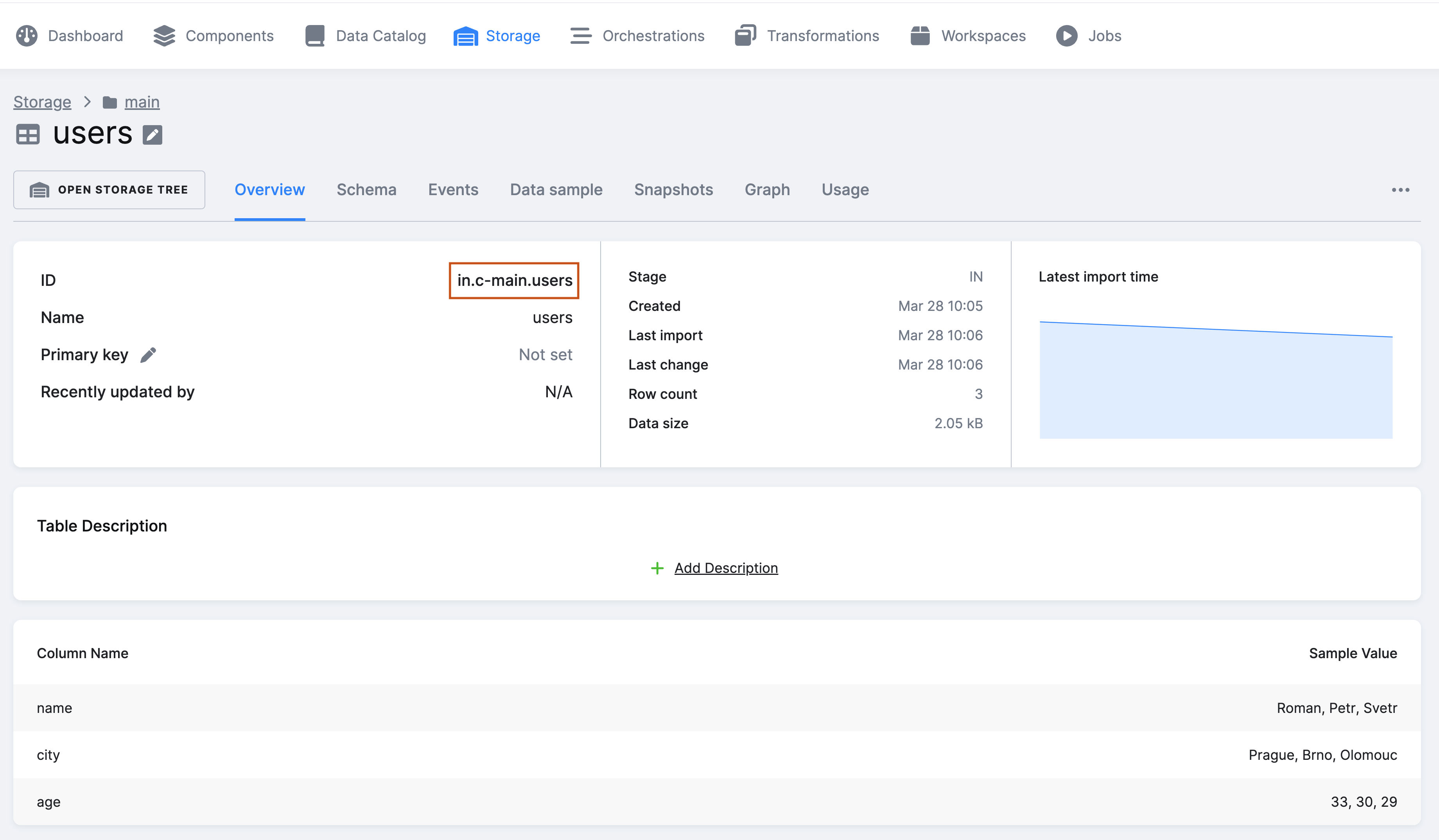
You have read access to all the tables in your project’s Storage directly on the underlying backend. However, this means you need to use the internal ID of a bucket (in.c-main instead of main as you see in the UI).
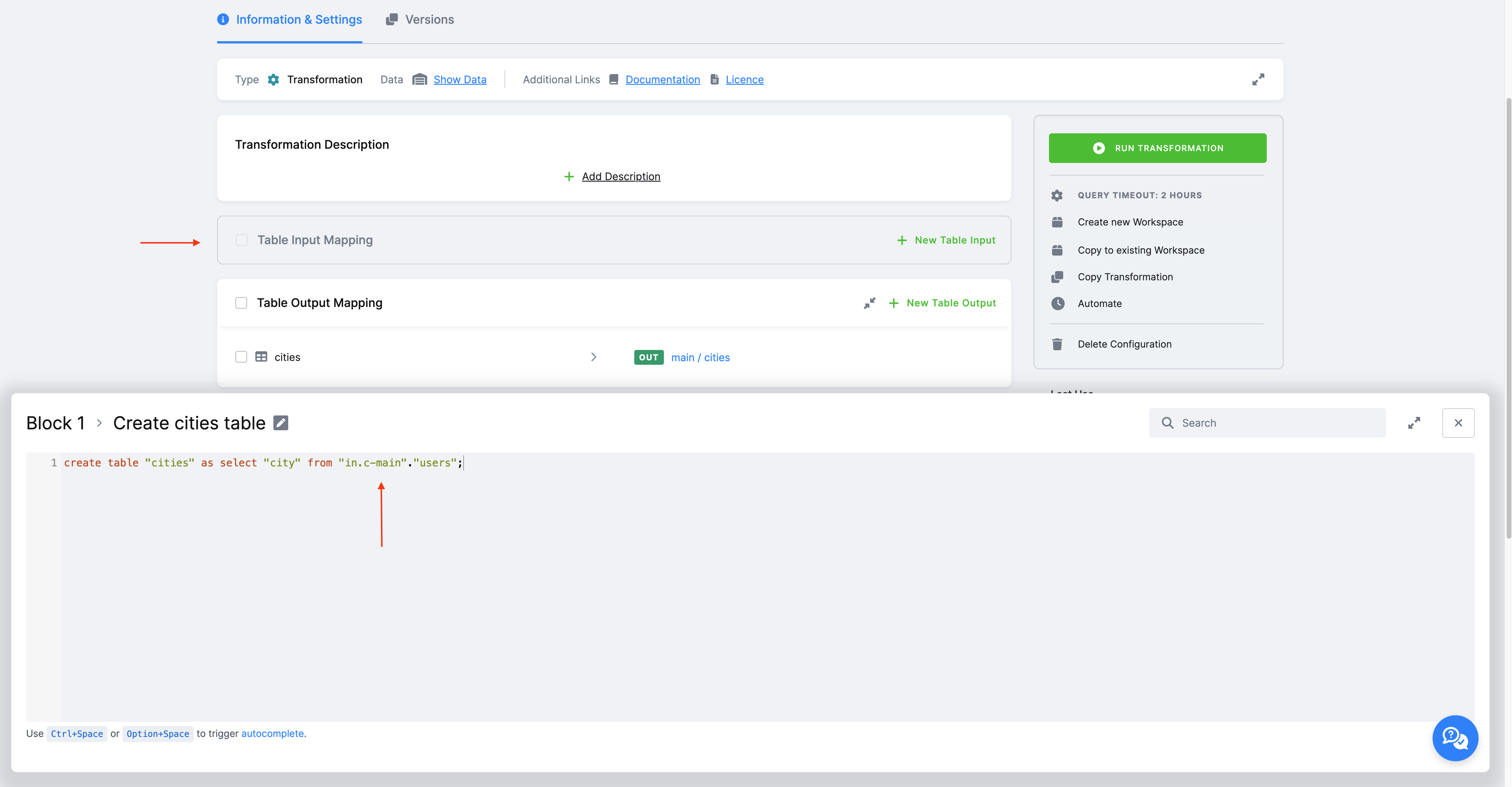
In the transformation code (Snowflake), we select from the table “in.c-main”.”users” and create a new table: create table "cities" as select "city" from "in.c-main"."users";.
Depending on the backend, the SQL format is different. More info regarding access to individual tables depending on the backend can be found in the documentation of those individual backends ( Snowflake, BigQuery ).
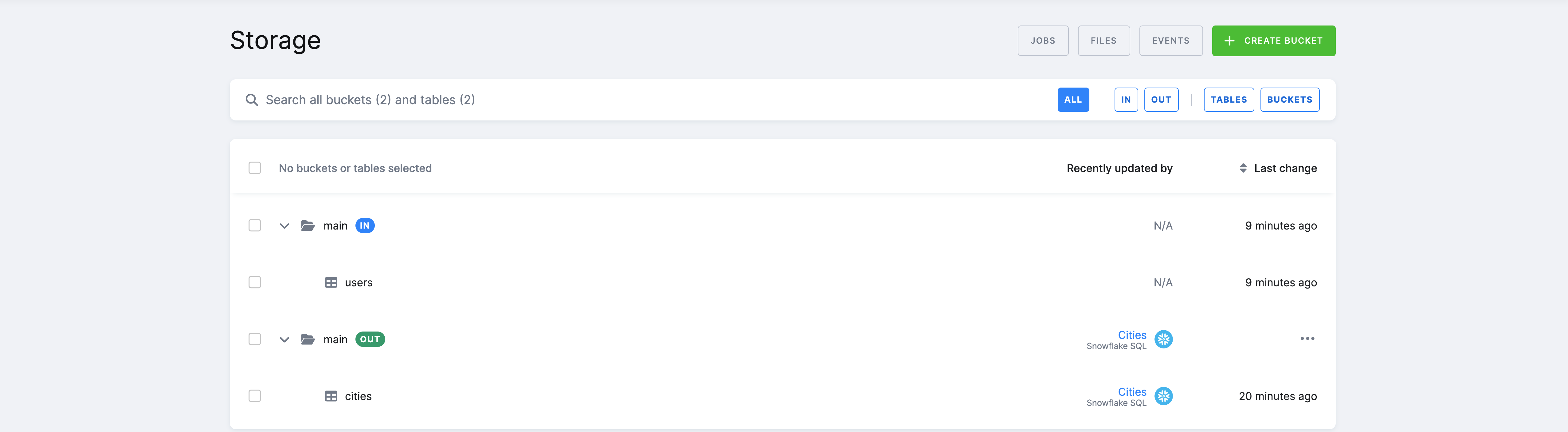
As you can see, a read-only input mapping allows you to read a table created in Storage directly in the transformation.
_timestamp system column
A table loaded using CLONE will contain all columns of the original table plus a new _timestamp column.
This column is used internally by Keboola for comparison with the value of the Changed in last filter.
The value in the column contains a unix timestamp of the last change of the row. You can use this column to set up incremental processing, i.e., to replace the role of the Changed in Last filter in the input mapping (which you can’t use with a clone mapping).
Important: The _timestamp column cannot be imported back to Storage.
When you attempt to do so, you’ll get the following error:
Failed to process output mapping: Failed to load table "out.c-test.opportunity":
Invalid columns: _timestamp: Only alphanumeric characters and underscores are allowed in the column name.
Underscore is not allowed on the beginning.
If you are not using the _timestamp column in your transformation, you have to drop it, for example:
`ALTER TABLE "my-table" DROP COLUMN "_timestamp";`
The _timestamp column is not present on tables loaded using the copy method.
File Input Mapping
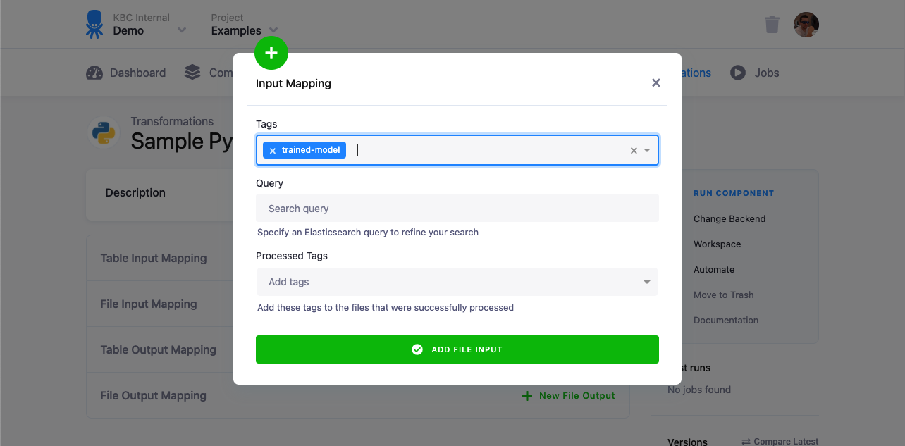
The file input mapping process exports the selected files from file Storage and copies them to the staging Storage. Depending on the transformation, this can be either a drive local to the transformation or a remote storage such as Amazon S3 or Azure Blob Storage. A file input mapping cannot operate with storage tables, but it comes in handy for processing files that cannot be converted to tables (binary files, malformed files, etc.) or, for example, to work with pre-trained models that you can use in a transformation.
Options
- Tags — specify tags which will be used to select files.
- Query — if selecting files by tags is not precise enough, you can use an elastic query to refine the search. If you combine query with tags, both conditions must be met.
- Processed Tags — specify tags which will be assigned to the input files once the transformation is finished. This allows you to process Storage files in an incremental fashion. You can combine this setting with the query option to omit already processed files in recurring transformations.
Output Mapping
An output mapping takes results (tables and files) from your transformation and stores them back in Storage.
It can create, overwrite, and append any table.
These tables are typically derived from the tables/files in the input mapping. In SQL transformations,
you can use any CREATE TABLE, CREATE VIEW, INSERT, UPDATE or DELETE queries to create the desired result.
The result of output mapping can be both Storage tables and Storage files. The common first choice is to use the table output mapping. The rule is that any tables or files not specified in the output mapping are considered temporary and are deleted when the transformation job ends. You can use this to your advantage and simplify the transformation script implementation (no need to worry about cleanup or intermediary steps).
Keep in mind that every table or file specified in the output mapping must be physically present in the staging area. A missing source table for the output mapping is an error. This is important when the results of a transformation are empty — you have to ensure that an empty table or an empty file (with a header or a manifest) is created.
Table Output Mapping
Depending on the transformation backend, the table output mapping process can do the following:
- In case of Database Staging — copy the specified tables from the staging database into the project Storage tables.
- In case of File Staging — import the specified CSV files into project Storage tables.
The supported staging database type is Snowflake. The supported staging for CSV files is a storage local to the transformation.
See an example of setting up an output mapping in our tutorial.
Options
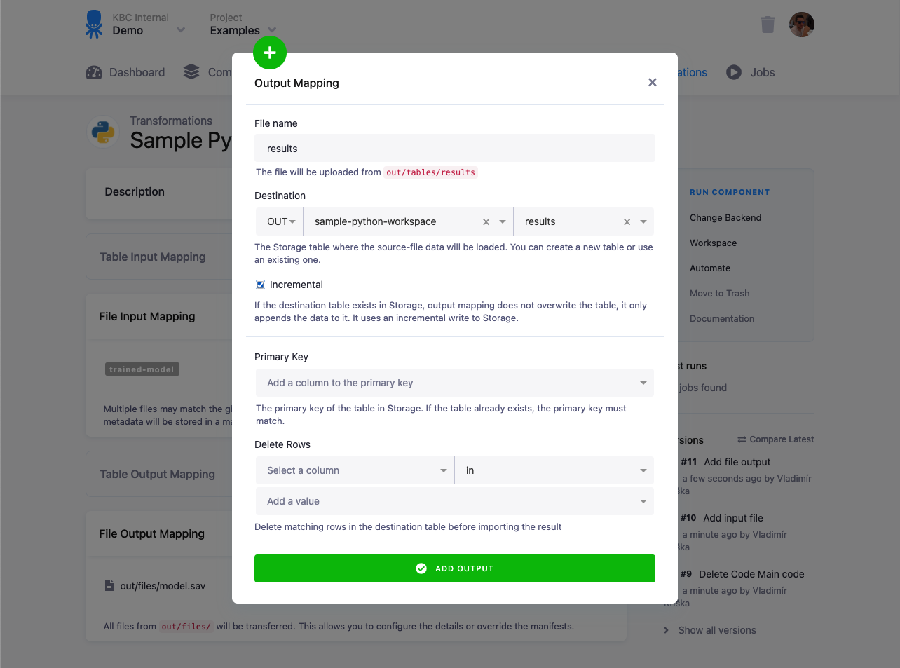
- Table — Enter the name of the table that should be created in the transformation.
- Destination — Select or type in the name of the Storage output table that will contain
the results of your transformation (i.e., contents of the Output Mapping source table).
- If this table does not exist yet, it will be created once the transformation runs.
- If this table already exists in Storage, the source table must match the structure of the destination table (all columns must be present, new columns will be added automatically).
- Incremental — Check this option to make sure that in case the Destination table already exists, it is not overwritten, but resulting data is appended to it. However, any existing row having the same primary key as a new row will be replaced. See the description of incremental loading for a detailed explanation and examples.
- Primary key — The primary key of the destination table; if the table already exists, the primary key must match. Feel free to use a multi-column primary key.
- Deduplication Strategy — This allows to switch in Snowflake transformations from the default load Upsert to Insert. Upsert option uses deduplication based on primary keys and ensures data quality. By switching to Insert, the load performs faster but skips deduplication and type casting - meaning you are responsible for uniqueness and correct data types. As this option is for high data maturity users, you can ask our support to enable this for your project as Deduplication Strategy is under feature flag.
- Delete rows — When Incremental loading is enabled, you can delete specific rows from the destination table before importing new data into the Storage. This gives you precise control over incremental updates. There are 2 options you can use:
- Delete rows from values - this option lets you manually specify values that identify rows to be removed from your destination table. This is particularly useful when the rows to delete are consistent, predictable, or rarely changing.
- Delete rows from transformation table - this option enables you to define deletion criteria using live data generated in your transformation.
This method provides flexibility for more complex, data-driven scenarios, such as removing obsolete records based on recent transactions or other dynamic conditions. This option needs to be enabled by navigating to Project Settings → Features → Delete rows from transformation table. Please note that this option is available in the production environment only and is not supported in development branches (e.g. for testing or configuration changes in a development branch, the option will not be applied).
- How the Delete Rows feature Works
DELETEstatements: - Each deletion query you configure creates a separate SQLDELETEstatement:- Multiple filters within a single query combine into a single```sql DELETE FROM table_name WHERE condition; ```DELETEwithANDconditions:- Multiple queries result in separate```sql DELETE FROM table_name WHERE condition1 AND condition2 AND ...; ```DELETEstatements, functioning as logicalOR:In this scenario, rows matching any of the specified conditions across the queries will be deleted.```sql DELETE FROM table_name WHERE condition1; DELETE FROM table_name WHERE condition2; ```Note: This process enables advanced row-level deletion logic, suitable for dynamic datasets where conditions may change per run.
Important: Multiple output mappings can be created for your transformation. Each source table can be used only once however.
File Output Mapping
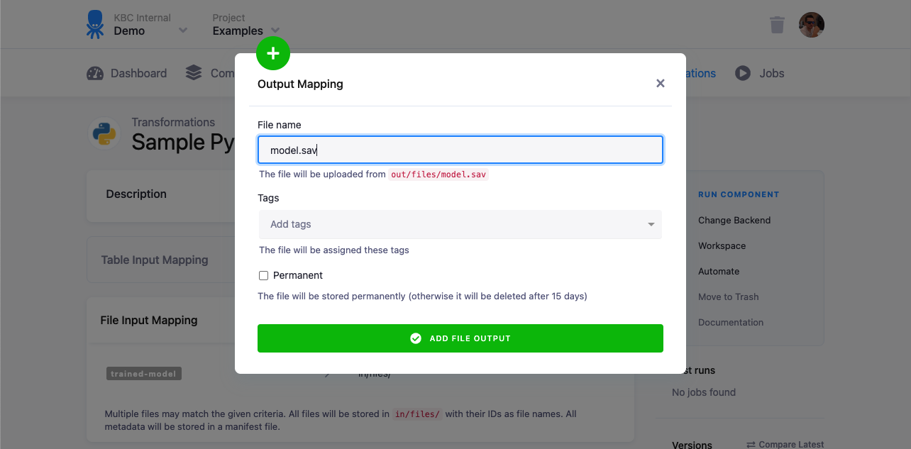
A file output mapping is used to store files produced by the transformation as Storage files. If you want to store CSV files as Storage tables, use table output mapping.
A file output mapping can be useful when your transformation produces, for example, trained models that are to be used in another transformation.
Only the files stored directly in the out/files/ directory can be mapped, subdirectories are not supported
(out/files/file.txt will work, out/files/subdir/file.txt won’t).
Options
- Source — Name of the source file for mapping
- Tag — Tags which will be applied to the target file uploaded in Storage
- Permanent - This option makes the file stay in the file Storage, until you delete it manually. If unchecked, the target file will be deleted after 15 days.